Diff for "HLS091828" - www.iram.es Main Wiki

Differences between revisions 1 and 43 (spanning 42 versions)

Brief analysis of the faint source HLS091828 (z=5.243)

Coordinates:

R.A. = 09h18m28.6s
Dec. = 51d42'23.3"

Expected luxes (Combes et al. 2012):

F1.3sma= 55+-7mJy
F0.88mm= 125+-8mJy
F2mm= 15+-7mJy

NIKA obsevations:

Day: 13/06/2013
Scans: 9 Lissajous of 5 min (<=> 45 min) each with followed by tracks (for tuning), 180 to 197
Size of the map:90"x90"
We detect the source at both wavelenghts, shown on the maps given bellow.
1mm_map.pdf 2mm_map.pdf
The profiles are computed by averaging the map in concentric annuli, and we check that the measured flux is, a priori, consistent with what we expect.

{{attachment:1mm_profile.png

width=550,height=400

1mm_profile.png}}

{{attachment:2mm_profile.png

width=550,height=400

2mm_profile.png}}

1mm_profile.pdf

2mm_profile.pdf
The time per pixel maps are also shown
1mm_time.pdf 2mm_time.pdf
Using Jack-Knives maps, we are able to estimate the noise level in the data.

-  ⇤ ← Revision 1 as of 2013-06-14 13:41:36 → 
  Size: 90
  Editor: NikaBolometer
  Comment:
+   ← Revision 43 as of 2013-06-14 15:52:31 → ⇥
  Size: 1344
  Editor: NikaBolometer
  Comment:
-Deletions are marked like this.
+Additions are marked like this.
 Line 1:
-Rédiger « HLS091828 » ici.
+'''Brief analysis of the faint source HLS091828 (z=5.243)'''
 Line 3:
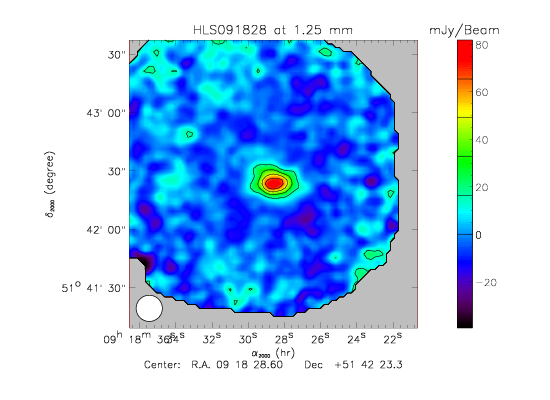
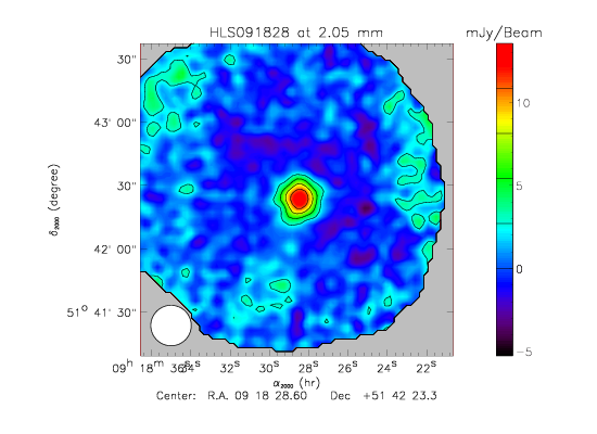
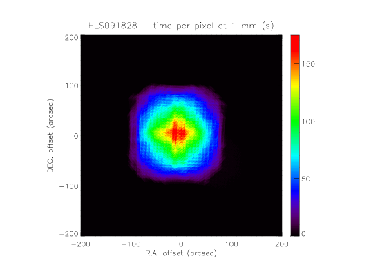
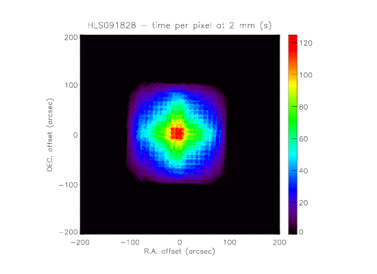
-Brief analysis of the faint source HLS091828 (z=5.243).
+'''''Coordinates:'''''
 .R.A. = 09h18m28.6s  
 .Dec. = 51d42'23.3"  

'''''Expected luxes (Combes et al. 2012): '''''
 .F1.3sma= 55+-7mJy
 .F0.88mm= 125+-8mJy
 .F2mm= 15+-7mJy

'''''NIKA obsevations:'''''
 .''Day:'' 13/06/2013
 .''Scans'': 9 Lissajous of 5 min (<=> 45 min) each with followed by tracks (for tuning), 180 to 197
 .''Size of the map'':90"x90"
 .We detect the source at both wavelenghts, shown on the maps given bellow. 
 {{attachment:1mm_map.png||width=550,height=400}}  {{attachment:2mm_map.png||width=550,height=400}}
 [[attachment:1mm_map.pdf]]  [[attachment:2mm_map.pdf]]


 .The profiles are computed by averaging the map in concentric annuli, and we check that the measured flux is, a priori, consistent with what we expect.

 || {{attachment:1mm_profile.png||width=550,height=400||1mm_profile.png}} ||  {{attachment:2mm_profile.png||width=550,height=400||2mm_profile.png}} ||
 || [[attachment:1mm_profile.pdf]] || [[attachment:2mm_profile.pdf]] ||

 .The time per pixel maps are also shown
 {{attachment:1mm_time.png||width=550,height=400}}  {{attachment:2mm_time.png||width=550,height=400}}
 [[attachment:1mm_time.pdf]]  [[attachment:2mm_time.pdf]]

 .Using Jack-Knives maps, we are able to estimate the noise level in the data.

{{attachment:1mm_profile.png	width=550,height=400	1mm_profile.png}}	{{attachment:2mm_profile.png	width=550,height=400	2mm_profile.png}}
1mm_profile.pdf	2mm_profile.pdf