|
Size: 4195
Comment:
|
Size: 7134
Comment:
|
| Deletions are marked like this. | Additions are marked like this. |
| Line 1: | Line 1: |
| ##acl NicolasBillot,hermelo,CarstenKramer,SamuelLeclerc:read,write,delete,revert,admin Default | ##acl hermelo,CarstenKramer,NicolasBillot,SamuelLeclerc:read,write,delete,revert,admin Default |
| Line 4: | Line 4: |
The following diagram shows the NIKA data flow from the IRAM 30m telescope to the observers' accounts. {{attachment:NIKApipeline.png | Neel Pipeline| height=600}} |
|
| Line 11: | Line 15: |
| == Getting ready == | == Offline data reduction == === Data products v0 === The version v0 of the NIKA first open pool products has been made by the NIKA team by the end of the pool (Feb 28,2014) and it was distributed by IRAM. The products are described [[attachment:NikaDataProductsV1.pdf | here ]]. For each project, there are fits files containing the maps of each scan and combined scans of each object. The data processing has been oriented towards point-source extraction or diffuse emission depending on the aim of your project. There are also logbook files and illustrative pdf files. On the main directory you will find: * '''logfile_all_scans.csv''': is a comma separated file ready for your favorite spreadsheet handler (libreoffice or excel). It gives the summary information of all the scans that could be used including opacity measurements, sky noise in Jy (per band of frequency from 1mHz to 10 Hz), camera noise NEFD (in mJy.s^1/2) and finally a flux in mJy of a point-source at the center of the map (fixed central position, fixed FWHM, Gaussian fit) with the error at both wavelengths. Then for each object, there is a directory that contains: * the '''fits''' files. * '''flux_source.csv''': a comma separated file giving the flux as measured in the scan maps and the combined scans maps. * '''Figures''': many pdf files were generated out of the fits files to get a quick look at them. Units in Jy. '''CAVEAT:''' At this stage, the data offline products are not of scientific quality. The selection of scans was unfortunately rendered difficult because of an unexpected problem with the pointing data. We hope to solve that problem with post-processing steps that we did not have time to implement. Instead, scans were manually selected with some mistakes still present. The photometry is probably correct at the 20% level at 1mm and 10% level at 2mm for scans of good quality. Don't shoot. We will prepare the next version in the coming weeks. Contact your NIKA friend of project to give us your feedback. ''The NIKA team'' |
| Line 14: | Line 56: |
| === Data products v1 === Coming soon... === Data products v2 === Coming (not so) soon... ---- == Online data reduction == |
|
| Line 15: | Line 69: |
| analaysis. | |
| Line 20: | Line 73: |
| > rt > emacs & |
|
| Line 25: | Line 76: |
| Shortly after a scan is done, the NIKA scientific data and the AntennaIMBfits are written on SAMI and can be processed. | Shortly after a scan is done, the NIKA scientific data, the xml information generated by PAKO (and the AntennaIMBfits shortly after) are written on SAMI and can be processed. |
| Line 30: | Line 80: |
| == Calibration scans == | === Calibration scans === |
| Line 32: | Line 82: |
| The calibration scans expect actions from the observer and interaction with !PaKo. | All calibration scans are reduced by the same routine: |
| Line 34: | Line 84: |
| === cont_pointing_cross === | '''IDL> rta_reduce, day, scan_num''' |
| Line 36: | Line 86: |
| * In the emacs window, edit run pointing.pro and update the day and scan num parameters. * update the p2cor and p7cor parameters with the “SET POINTING” values displayed in the PAKO window. * Save the file * In the idl session in T2, type .r run pointing * Several plot windows might be on top of eachother * Follow instructions returned by the code in T2. By default, follow instructions “B (2mm) : (MAP) (for PAKO and pointing model)”. |
'''day is in the format YYYYMMDD, e.g. 20140218, scan_num is a simple integer.''' |
| Line 43: | Line 88: |
| === cont_pointing_liss === * In the emacs window, edit run pointing liss.pro and update the day and scan num parameters. * Save the file * In the idl session in T2, type .r run pointing liss * Several plot windows might be on top of eachother * Follow instructions returned by the code in T2 === cont_focus_track === * In the emacs window, edit run focus.pro and update the day and scan num parameters. * Check the value of focusz in the PAKO display window. * Do not change the fooffset values unless you have modified the pako script focusp.pako. * Save the file * In the idl session in T2, type .r run focus * Several plot windows might be on top of eachother * Follow instructions returned by the code in T2 === cont_focus_liss === * In the emacs window, edit run focus liss.pro and update the day and scan num parameters. Scan num should be the first of the five scans involved in this analysis. * Save the file * In the idl session in T2, type .r run focus liss * Several plot windows might be on top of eachother * Follow instructions returned by the code in T2 === cont_skydip === * In the emacs window, edit run skydip.pro and update the day and scan num parameters. * Save the file * In the idl session in T2, type .r run skydip * Several plot windows might be on top of eachother * Follow instructions returned by the code in T2 === cont_beammap === * In the emacs window, edit run otf geometry.pro and update the day and scan num parameters. * Save the file * In the idl session in T2, type .r run otg geometry * Several plot windows might be on top of eachother * Follow instructions returned by the code in T2 |
Informations or actions to be taken by the observer appear on the plots and explicitely in IDL terminal window: |
| Line 86: | Line 91: |
| == Science scans == | ==== cont_pointing_cross ==== |
| Line 88: | Line 93: |
| The science scans are meant to be optimally processed offline with tailored procedures. The real time software mentioned in this note only aims at giving a quick feedback | {{attachment:cross.png||width=400}} |
| Line 90: | Line 95: |
| === Total power maps === | * The plots show 1D profiles of the azimuth or elevation scans at both wavelenght for the reference detector and a gaussian fit of the source along the timeline. The displayed offsets refer to the reference detectors and are not meant to be passed to PAKO. * The maps show the source, a cross at the location of the reference pixel and gaussian fit of the source * In the terminal window, the observer should follow the instruction (e.g.): B 2mm (MAP) (for PAKO) SET POINTING 3.0 0.7 * the pointing reference is the 2mm channel. * If the sky conditions were correct, instructions at 1 and 2mm should be in good agreement. * if a glitch corrupts the maps but the 1d profiles are ok, the user can follow the instruction B 2mm, : (TOI) (for PAKO) SET POINTING 3.0 0.7 * In good conditions, all instructions agree to better than 1 arcsec. * If the pointing is far off, the default reference pixels may not see the source and the timelines may look bad. In the terminal window, you may read the ID of the closest kids to the source and pass them to rta_reduce as keywords e.g. '''rta_reduce, day, scan_num, numdet1=5, numdet2=494''' |
| Line 92: | Line 104: |
| All maps (cont_onthefly and cont_lissajous) in total power mode can be reduced by the same script: | |
| Line 94: | Line 105: |
| * In the emacs window, edit run otf map.pro and update the scan num and day parameters. * If you’re observing a point source, set diffuse = 0. If you’re observing diffuse emission set diffuse = 1. * Save the file * In the idl session in T2, type .r run otf map * Several plot windows might be on top of each other |
==== cont_pointing_liss ==== |
| Line 100: | Line 107: |
| === Polarization maps === | {{attachment:pointing_liss.png||width=400}} |
| Line 102: | Line 109: |
| All maps (OTF or Lissajou) in Polarization modes can be reduced by the same script: | * The routine displays one map for each band, an estimation of the flux where the source is fit (red), an estimation of the flux at the center of the map (green). It also provides a quick estimate of the NEFD and the map RMS for 10arcsec equivalent pixels and the values of Tau derived by NIKA. * The observer should follow instructions given in the terminal, e.g.: B 2mm, : (MAP) (for PAKO) SET POINTING -4.7, 1.4 |
| Line 104: | Line 112: |
| * In the emacs window, edit run otf polar maps.pro and update the scan num and day parameters. * Save the file * In the idl session in T2, type .r run otf polar maps * Several plot windows might be on top of each other |
==== cont_focus_track ==== {{attachment:focus.png||width=400}} * you may change the reference kids as before e.g. '''rta_reduce, day, scan_num, numdet1=5, numdet2=494''' * By default, optimize the focus at 1mm ==== cont_skydip ==== {{attachment:skydip_results.png||width=400}} * No action is requested from the observer other than checking that the displayed histograms look reasonable. These results will be used by the NIKA team later on offline. ==== cont_focus_liss ==== {{attachment:pointing_liss.png||width=400}} {{attachment:fits.png||width=400}} * As soon as the data of a scan of this sequence are on Sami's disk, you may run '''rta_reduce, day, scan_num''' * When at least 3 of the 5 scans are done, you may call '''focus_liss, day, [scan_num1, scan_num2, scan_num3]''' to have a first guess of the optimal focus * When the 5 scans are done, call focus_liss with the complete list of scans and follow instructions in the terminal window and by default, optimize the focus at 1mm ==== cont_beammap ==== {{attachment:otf_geometry.png||width=400}} * Instead of rta_reduce, please call '''otf_geometry, day, scan_num''' * The top plots compare the current derived beam maps to the reference ones * The bottom plots display the distance between the current beam parameters and the reference ones in terms of centroids positions, FWHM and absolute calibration. === Science scans === ==== Point source maps ==== * rta_reduce, day, scan_num * If you want to coadd several scans, run '''combine_scans, scan_list'''. Note however that to allow to combine scans from different days, scan_list is here defined slightly differently, it is an array of strings of the format ''YYYYMMDDsScan_num'', e.g. '20140127s290' === Diffuse emission === * rta_reduce, day, scan_num, /diffuse * to combine several scans, use combine_scans in the same way as for point source maps |
| Line 110: | Line 162: |
Author: Israel Hermelo (IRAM 30m continuum pool manager) email: hermelo@iram.es Created: 2014.02.06 Last update: 2014.02.06 |
NIKA Data Reduction
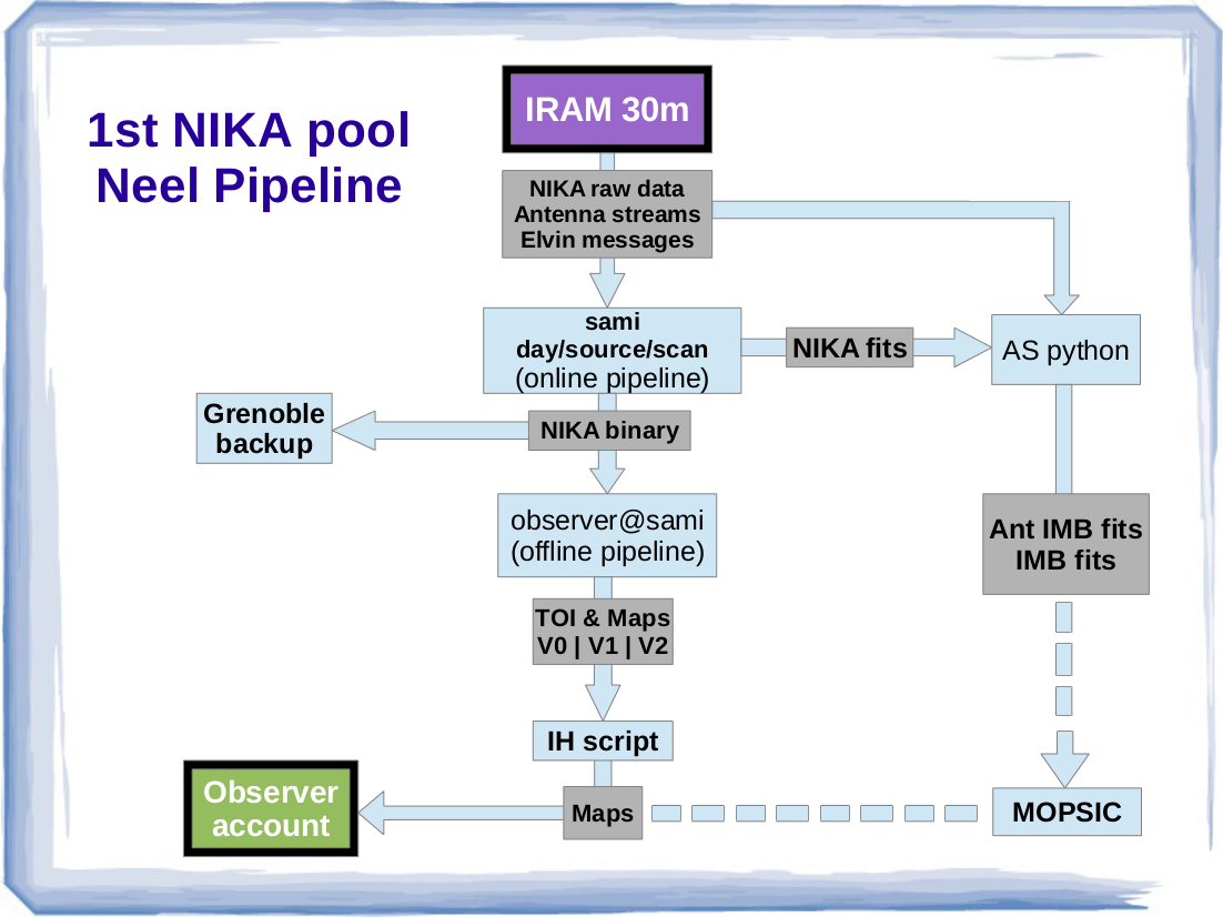
The following diagram shows the NIKA data flow from the IRAM 30m telescope to the observers' accounts.
Contents
Offline data reduction
Data products v0
The version v0 of the NIKA first open pool products has been made by the NIKA team by the end of the pool (Feb 28,2014) and it was distributed by IRAM. The products are described here.
For each project, there are fits files containing the maps of each scan and combined scans of each object. The data processing has been oriented towards point-source extraction or diffuse emission depending on the aim of your project.
There are also logbook files and illustrative pdf files. On the main directory you will find:
logfile_all_scans.csv: is a comma separated file ready for your favorite spreadsheet handler (libreoffice or excel). It gives the summary information of all the scans that could be used including opacity measurements, sky noise in Jy (per band of frequency from 1mHz to 10 Hz), camera noise NEFD (in mJy.s^1/2) and finally a flux in mJy of a point-source at the center of the map (fixed central position, fixed FWHM, Gaussian fit) with the error at both wavelengths.
Then for each object, there is a directory that contains:
the fits files.
flux_source.csv: a comma separated file giving the flux as measured in the scan maps and the combined scans maps.
Figures: many pdf files were generated out of the fits files to get a quick look at them. Units in Jy.
CAVEAT: At this stage, the data offline products are not of scientific quality. The selection of scans was unfortunately rendered difficult because of an unexpected problem with the pointing data. We hope to solve that problem with post-processing steps that we did not have time to implement. Instead, scans were manually selected with some mistakes still present. The photometry is probably correct at the 20% level at 1mm and 10% level at 2mm for scans of good quality. Don't shoot. We will prepare the next version in the coming weeks. Contact your NIKA friend of project to give us your feedback.
The NIKA team
Data products v1
Coming soon...
Data products v2
Coming (not so) soon...
Online data reduction
To start the IDL session for the real time analysis, open a terminal and type:
   $ ssh -X nikaw-13@mrt-lx1
   $ ssh_sami
   > idl
Shortly after a scan is done, the NIKA scientific data, the xml information generated by PAKO (and the AntennaIMBfits shortly after) are written on SAMI and can be processed. There are two types of observation: the “science” scans and the “calibration” scans. There is a specific routine to analyze each type of scan.
Calibration scans
All calibration scans are reduced by the same routine:
IDL> rta_reduce, day, scan_num
day is in the format YYYYMMDD, e.g. 20140218, scan_num is a simple integer.
Informations or actions to be taken by the observer appear on the plots and explicitely in IDL terminal window:
cont_pointing_cross
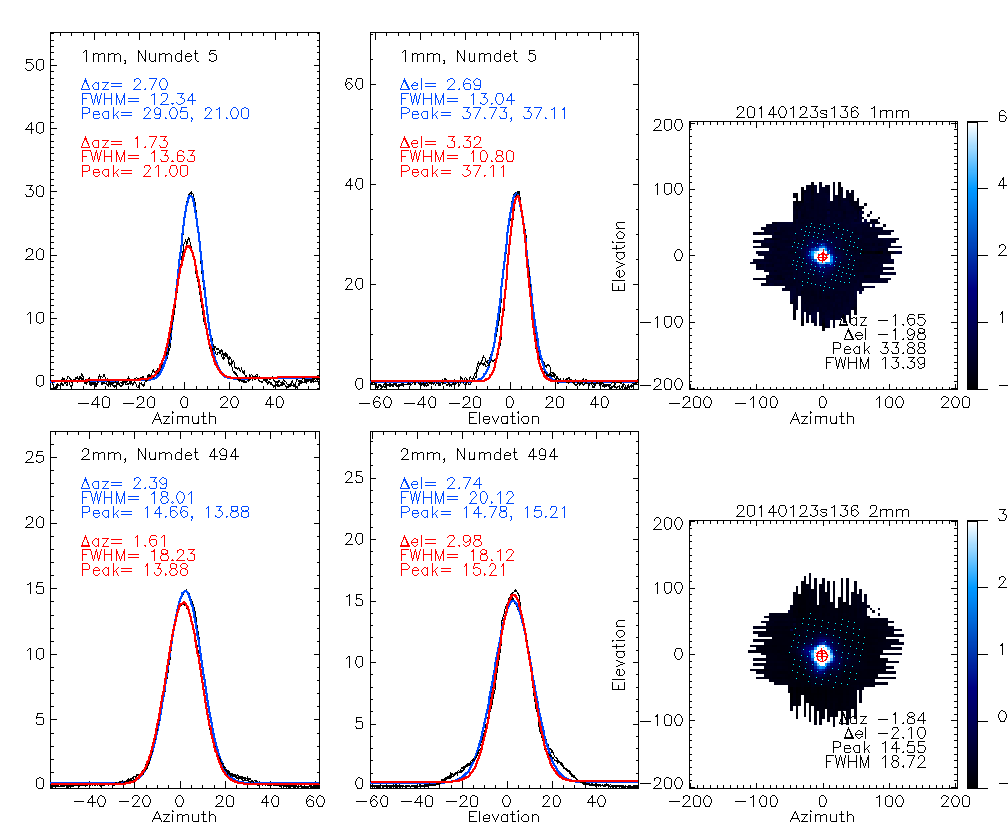
- The plots show 1D profiles of the azimuth or elevation scans at both wavelenght for the reference detector and a gaussian fit of the source along the timeline. The displayed offsets refer to the reference detectors and are not meant to be passed to PAKO.
- The maps show the source, a cross at the location of the reference pixel and gaussian fit of the source
- In the terminal window, the observer should follow the instruction (e.g.): B 2mm (MAP) (for PAKO) SET POINTING 3.0 0.7
- the pointing reference is the 2mm channel.
- If the sky conditions were correct, instructions at 1 and 2mm should be in good agreement.
- if a glitch corrupts the maps but the 1d profiles are ok, the user can follow the instruction B 2mm, : (TOI) (for PAKO) SET POINTING 3.0 0.7
- In good conditions, all instructions agree to better than 1 arcsec.
If the pointing is far off, the default reference pixels may not see the source and the timelines may look bad. In the terminal window, you may read the ID of the closest kids to the source and pass them to rta_reduce as keywords e.g. rta_reduce, day, scan_num, numdet1=5, numdet2=494
cont_pointing_liss
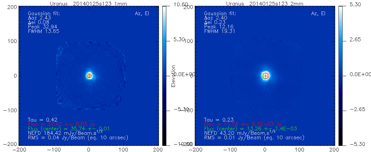
- The routine displays one map for each band, an estimation of the flux where the source is fit (red), an estimation of the flux at the center of the map (green). It also provides a quick estimate of the NEFD and the map RMS for 10arcsec equivalent pixels and the values of Tau derived by NIKA.
- The observer should follow instructions given in the terminal, e.g.: B 2mm, : (MAP) (for PAKO) SET POINTING -4.7, 1.4
cont_focus_track
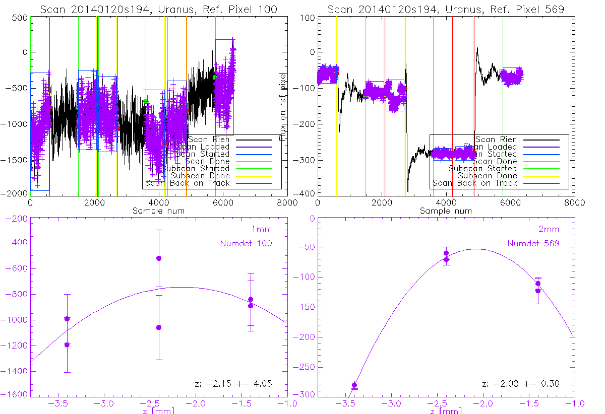
you may change the reference kids as before e.g. rta_reduce, day, scan_num, numdet1=5, numdet2=494
- By default, optimize the focus at 1mm
cont_skydip
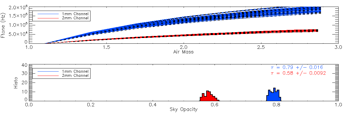
- No action is requested from the observer other than checking that the displayed histograms look reasonable. These results will be used by the NIKA team later on offline.
cont_focus_liss

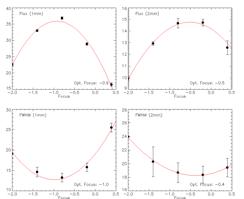
As soon as the data of a scan of this sequence are on Sami's disk, you may run rta_reduce, day, scan_num
When at least 3 of the 5 scans are done, you may call focus_liss, day, [scan_num1, scan_num2, scan_num3] to have a first guess of the optimal focus
- When the 5 scans are done, call focus_liss with the complete list of scans and follow instructions in the terminal window and by default, optimize the focus at 1mm
cont_beammap
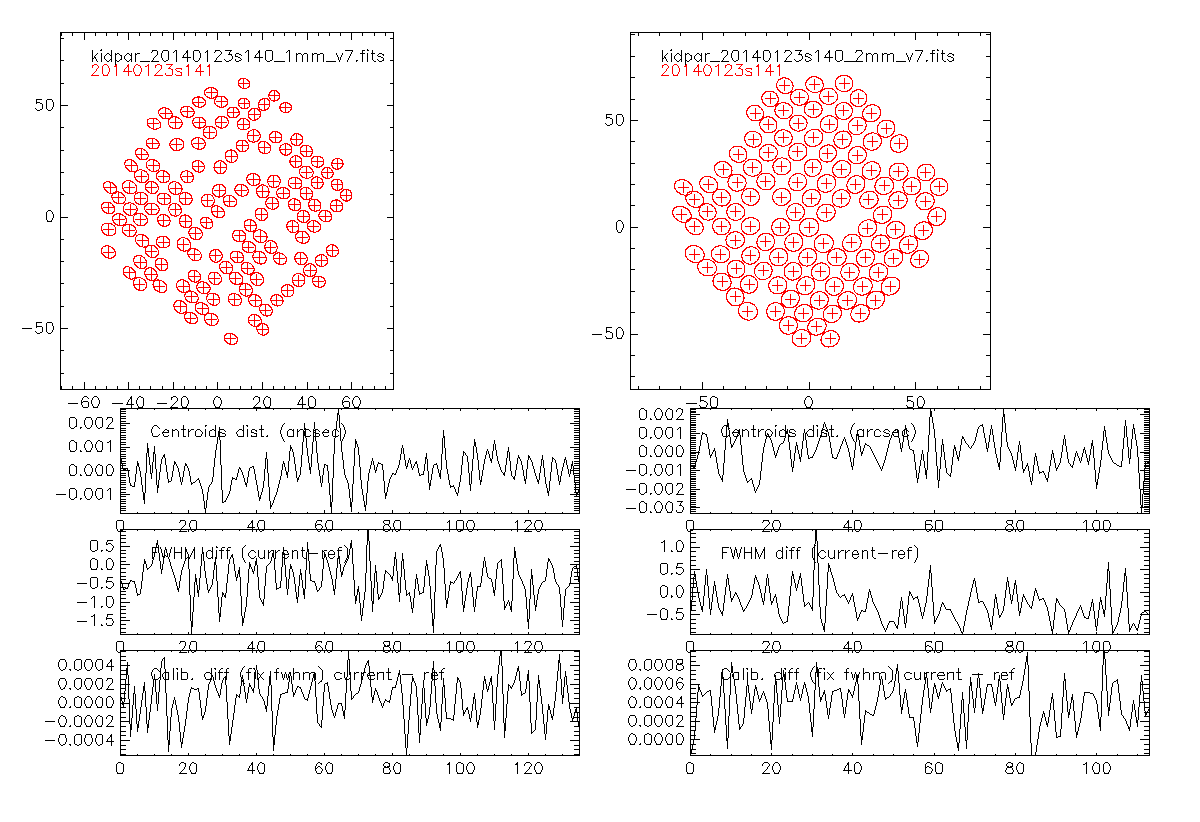
Instead of rta_reduce, please call otf_geometry, day, scan_num
- The top plots compare the current derived beam maps to the reference ones
- The bottom plots display the distance between the current beam parameters and the reference ones in terms of centroids positions, FWHM and absolute calibration.
Science scans
Point source maps
- rta_reduce, day, scan_num
If you want to coadd several scans, run combine_scans, scan_list. Note however that to allow to combine scans from different days, scan_list is here defined slightly differently, it is an array of strings of the format YYYYMMDDsScan_num, e.g. '20140127s290'
Diffuse emission
- rta_reduce, day, scan_num, /diffuse
- to combine several scans, use combine_scans in the same way as for point source maps
